Download Postscript File

Download Compressed Postscript File

Application of the Quasi-Inverse Method
to Data Assimilation

Eugenia Kalnay^1,2,3,, Seon Ki Park², Zhao-Xia Pu¹ and Jidong Gao<sup>4

1</sup>National Centers for Environmental Prediction
NWS/NOAA, Washington, D.C. 20233

²Cooperative Institute for Mesoscale Meteorological Studies
³School of Meteorology
⁴Center for Analysis and Prediction of Storms
University of Oklahoma, Norman, OK 73019


December 1998 (Revised)


Submitted to Monthly Weather Review.

ABSTRACT

Four-dimensional variational data assimilation (4D-Var) seeks to find an optimal initial field that minimizes a cost function defined as the squared distance between model solutions and observations within an assimilation window. For a perfect linear model, Lorenc showed that the 4D-Var forecast at the end of the window coincides with a Kalman Filter analysis if two conditions are fulfilled: a) the addition to the cost function of a term that measures the distance to the background at the beginning of the assimilation window, and b) the use of the Kalman Filter background error covariance in this term. The standard 4D-Var requires minimization algorithms along with adjoint models to compute gradient information needed for the minimization. In this study, we suggest that an alternative method based on the use of the quasi-inverse model that, for certain applications, may help accelerate the solution of problems close to 4D-Var.

We introduce the quasi-inverse approach for the forecast sensitivity problem, and then formulate a closely related variational assimilation problem using the quasi-inverse model (i.e., the model integrated backwards but changing the sign of the dissipation terms). We show that if the cost function has no background term, and has a complete set of observations (as assumed in many classical 4D-Var papers), the new method solves the 4D-Var-minimization problem efficiently, and is in fact equivalent to the Newton algorithm but without having to compute a Hessian. If the background term is included but computed at the end of the interval, allowing the use of observations that are not complete, the minimization can still be carried out very efficiently. In this case, however, the method is much closer to a 3D-Var formulation in which the analysis is attained through a model integration. For this reason, we call the method ``Inverse 3D-Var'' (I3D-Var).

We applied the I3D-Var method to simple models (Burgers' equation and Lorenz model), and found that when the background term is ignored and complete fields of noisy observations are available at multiple times, the Inverse 3D-Var method minimizes the same cost function as 4D-Var but converges much faster. Tests with the Advanced Regional Prediction System (ARPS), indicate that I3D-Var is about twice as fast as the Adjoint Newton Method and many times faster than the quasi-Newton LBFGS algorithm, which uses the adjoint model. Potential problems (including the growth of random errors during the integration back in time) and possible applications to problems such as storm-scale data assimilation and reanalysis are also discussed.

1. Introduction

Over the last decade many important applications of the backward integration of the adjoint of the linear tangent model have been introduced in the literature. These include the generation of singular vectors for ensemble prediction (e.g., Molteni et al. 1996); four-dimensional variational data assimilation (e.g., Lewis and Derber 1985; Le Dimet and Talagrand 1986; Courtier et al. 1994); forecast sensitivity to the initial conditions (Rabier et al. 1996; Pu et al. 1997a); and targeted observations (e.g., Rohaly et al. 1998; Pu et al. 1998).

Among advanced methods for data assimilation, 4-dimensional Variational data assimilation (4D-Var) is the approach that has received the most attention in recent years (Derber 1989; Courtier et al. 1994; M. Zupanski 1993; and many other papers). A simplified version has been implemented recently at ECMWF (Bouttier and Rabier 1997; Rabier et al. 1997), and at the time of this writing, NCEP is testing a 4D-Var system for the Eta model.

In 4D-Var a cost function is defined as the squared distance between a model integration and the observations in a given assimilation interval. Lorenc (1986, 1988) showed that for a linear perfect model, if a) a background error term is added to the cost function at the beginning of the assimilation period, and b) the background error covariance is the same as that used in the Kalman Filter (KF) at the initial time, then the 4D-Var analysis at the end of the interval is the same that would be obtained using the KF. This makes 4D-Var attractive, because it is much less expensive than KF (see also Daley 1991, and Thepaut et al. 1993).

4D-Var provides initial conditions for a model integration that is close to the observations, but it also has some disadvantages: a) It is difficult to include forecast error covariances in the cost function except at the beginning of the interval, which forces the use of short assimilation intervals in order to maintain the impact of model errors small. It is obvious from Lorenz chaos theory that even with a perfect model, one would not want to perform 4D-Var over, for example, a two-week data assimilation interval, since the 4D-Var analysis would be given by the state of the model after a two-week integration, when the predictability has been lost (Pires et al. 1996). Even if the assimilation interval is reduced to a shorter period, such as 6-24 hours, the neglect of model errors during the forecast can lead to unrealistic results (Menard and Daley 1996). There have been attempts to include simple evolving model errors (e.g., Derber 1989; D. Zupanski 1997) but much remains to be done in this area. b) 4D-Var has a large computational cost compared to 3D-Var (typically 10-100 or more iterations are required for convergence, equivalent to about 30-300 model integrations per day). ECMWF, for example, has a powerful supercomputer about 25 times faster than a Cray C90, and has been running a model at a horizontal resolution of T213. Nevertheless, ECMWF had to make several simplifying assumptions in their implementation of 4D-Var (such as using a lower horizontal resolution model of T63 and a short assimilation window) in order to reduce the computational cost (Bouttier and Rabier 1997; Rabier et al. 1997).

Recently Wang et al. (1997) suggested the use of backward model integrations in order to accelerate the convergence of 4D-Var (without including background error in the cost function). Pu et al. (1997a) showed that for the problem of forecast sensitivity, closely related to 4D-Var, a backward integration with the ``quasi-inverse'' of the tangent linear model (TLM) gave results far superior to those obtained using the adjoint model. The quasi-inverse model is simply the model integrated backwards but changing the sign of dissipative terms in order to avoid computational blow-up. It can be applied to either the tangent linear or the full nonlinear model, each of which has advantages for different applications. The quasi-inverse linear (QIL) method has been tested successfully at NCEP in several different applications, e.g., forecast error sensitivity analysis and data assimilation (Pu et al. 1997a), and adaptive observations (Pu et al. 1998).

Wang et al. (1997) adopted the quasi-inverse approach for their adjoint Newton algorithm (ANA), and applied it to a simplified 4D-Var problem, using simulated data, using the Advanced Regional Prediction System (ARPS; Xue et al. 1995), with impressive results. They assumed the availability of a complete set of observations at the end of the assimilation interval, and showed that the ANA converged in an order of magnitude fewer iterations, and to an error level an order of magnitude smaller than the conventional adjoint approach to solve the same (simplified) 4D-Var problem.

Kalnay and Pu (1998) generalized Wang et al. (1997) approach by including a background term to the cost function and further simplified the method. The background error term in the cost function allows using incomplete sets of observations, but in order to maintain the efficiency of the method, it is necessary to estimate the background error term at the end of the assimilation interval, rather than at the beginning as in Lorenc (1986) formulation. We have further generalized the method to allow for the assimilation of data at different times, rather than only at the end of the interval, as in Wang et al. (1997). The results suggest that the quasi-inverse model may be used in data assimilation for accelerating convergence and reducing spin-up problems, although problems may arise when tested on comprehensive atmospheric models.

In this paper we first introduce the quasi-inverse approach for the forecast sensitivity problem, and then formulate a closely related variational assimilation problem using the quasi-inverse model (section 2). We show that if the cost function has no background term, and has a complete set of observations (as was assumed in many classical 4D-Var papers), the new method solves the 4D-Var-minimization problem efficiently, and is in fact equivalent to the Newton algorithm but without having to compute a Hessian. If the background term is included but computed at the end of the interval, the minimization can still be carried out very efficiently, but in this case it the method is closer to a 3D-Var formulation in which the analysis is attained through a model integration. For this reason, we call the method ``Inverse 3D-Var'' (I3D-Var).

In section 3 we introduce a simple ``model'' (viscous Burger's equation with advection of a passive scalar) which includes effects mimicking the three main components of atmospheric models: advection, large-scale instabilities, and dissipative processes. Using this simple model we show the effects of applying a linear tangent model, its adjoint, the exact inverse, and the quasi-inverse model, and compare one iteration of Inverse 3D-Var and adjoint 4D-Var. In section 4 we present preliminary results comparing Inverse 3D-Var and the adjoint 4D-Var using Burger's model and Lorenz's model (Lorenz 1963). We show that when the background term is ignored and complete fields of noisy observations are available at multiple times, the Inverse 3D-Var method still minimizes the same cost function as 4D-Var (but much more efficiently). Section 5 discusses several topics related to possible applications of Inverse 3D-Var: assimilation of data at multiple time levels, research on a storm-scale model with reversible clouds for storm-forecast initialization, and the problem of random observational errors which may amplify during the backward integration (Reynolds and Palmer 1998).

2. Formulation of Inverse 3D-Var

a. Forecast sensitivity

We introduce Inverse 3D-Var by first considering the forecast sensitivity problem posed by Rabier et al (1996): Find the change in initial conditions ${{\delta}x}$ that ``optimally'' corrects a perceived forecast error at the final time t. In what follows, M_t is a nonlinear forecast operator that advances the model state x from t = 0 to the final time t, i.e., x_t = M_t (x₀). A is the analysis, E = A_t - M_t (x₀) is the perceived error, L is the linear propagator (linear tangent model integrated forward in time), and L^T is its adjoint. Then ${{\delta}x}$ is the solution of

$$M_{t} (x_{0} + {{\delta}x}) = A_{t}$$ (1)

or

$$L{{\delta}x} \cong A_{t} - M_{t} (x_{0}) = E.$$ (2)

1) ADJOINT APPROACH (RABIER ET AL. 1996; PU ET AL. 1997B):

In the standard adjoint approach, we define a cost function using, for example, an energy norm (i.e., the energy of a vector y defined as (Wy)^T(Wy) = y^TW²y with W a weight matrix):

$$J = (WL{{\delta}x})^{T}WL{{\delta}x} = {{\delta}x}^{T}L^{T}W^{2}L{{\delta}x},$$ (3)

and compute its gradient

$${{\nabla}J} = L^{T}W^{2}L{{\delta}x} = L^{T}W^{2}E.$$ (4)

Equation (4) indicates that to obtain the gradient of the cost function we have to integrate backwards with the adjoint model, starting from the perceived error at the final time. This gives the ``optimal'' direction that results in the maximum decrease of the cost function for a given size perturbation. The adjoint procedure requires in addition an estimation of an appropriate amplitude $\alpha$, after which the adjoint sensitivity correction becomes

$${{\delta}x} = {\alpha}{{\nabla}J}.$$ (5)

This correction can be plugged into (1) and the whole procedure iterated (Pu et al. 1997a).

2) QUASI-INVERSE APPROACH:

In the Quasi-Inverse Linear (QIL) approach we try to solve (2) directly, but in order to do so, we need to have an approximation of the inverse of the TLM:

$${{\delta}x} = L^{-1}E.$$ (6)

The QIL approximation to L^-1 consists of simply running the TLM backward (changing the sign of ${\Delta}t$, and also changing the sign of the dissipative terms to avoid computational blow-up). Pu et al. (1997a) found that this is a rather accurate approximation to the inverse model. It solves a deterministic problem, so that there is no need to find an optimal amplitude, as required by the adjoint method. Reynolds and Palmer (1998) compared this method with running the exact inverse (using a Runge-Kutta time scheme and no change in sign for dissipation). They found that the presence of dissipation during the backward integration had a beneficial effect of a small reduction in noisiness.

Note that the inverse solution is not ``optimal'' like the adjoint solution, since there is no constraint on the size of ${{\delta}x}$. However, the inverse approach can be considered to be ``perfect'': it reaches in a single step the same solution (${{\nabla}J} \cong$ 0) that the adjoint approach would reach after many iterations. It should be pointed out that Lorenc (1988) integrated the NMC nested grid model (NGM) backward with a change of sign in the physics, but in his experiments he was attempting to approximate the adjoint model, not the inverse model.

b. Inverse 3D-Var

Wang et al. (1997) were trying to solve the 4D-Var problem on what they denote the ``estimated Newton descent direction'' rather than the descent direction provided by the standard adjoint approach. For this purpose they needed to approximate the inverse TLM, and succeeded by adopting the QIL method. In the experiments they did with simulated data and the adiabatic version of the ARPS model, they got convergence in an order of magnitude fewer iterations with the new method (ANA), and a decrease of the cost function which was also an order of magnitude better than with the adjoint approach. They assimilated simulated data only at the end of the interval, and only the full model field, so that they did not need a background error term in the cost function.

In this subsection we generalize their approach by including both data and background distance in the cost function, with appropriate error covariances. In order to maintain the ability to solve the minimization efficiently, however, the background term is estimated at the end of the interval, rather than at the beginning as in Lorenc (1986). Our derivation is also considerably simpler than the ANA method, and our method does not require line minimization, as in Wang et al (1997). As a result, our method is about twice as fast as the ANA approach.

Assume (for the moment) that data y^o is available at the end of the assimilation interval t, with ${{\delta}x}$=x^a-x^b, ${{\delta}y}$=y^o-$\mathsf{H}$(x^b). Here x^a and x^b are the analysis and first guess, respectively, and $\mathsf{H}$ is the ``forward observation operator'' which converts the model first guess into first guess observations (Ide et al. 1997). The cost function that we minimize is the 3D-Var cost function at the end of the interval. It is given by the distance to the background of the forecast at the end of the time interval (weighted by the inverse of the forecast error covariance B), plus the distance to the observations (weighted by the inverse of the observational error covariance R), also at the end of the interval:

$$J = \frac{1}{2}(L{{\delta}x})^{T}B^{-1}(L{{\delta}x}) + \fra... ...{{\delta}x}-{{\delta}y}]^{T}R^{-1}[HL{{\delta}x}-{{\delta}y}].$$ (7)

Here ${{\delta}x}$ (the control variable) is the difference between the analysis and the background (at the present iteration) at the beginning of the assimilation window, L and L^Tare, as before, the TLM and its adjoint, and H is the tangent linear version of the forward observation operator $\mathsf{H}$. If we take the gradient of J with respect to the initial change ${{\delta}x}$, we obtain

$${{\nabla}J} = L^{T}\{B^{-1}L{{\delta}x} + H^{T}R^{-1}[HL{{\delta}x}-{{\delta}y}]\}.$$ (8)

From this equation we see that the gradient of the cost function is given by the backward adjoint integration of the rhs terms in (8). In the adjoint 4D-Var, an iterative algorithm (such as quasi-Newton, conjugate gradient, or steepest descent) is used to estimate an optimum perturbation:

$${{\delta}x}^{i}={\alpha}_{i}{{\nabla}J}^{i-1}$$ (9)

and the procedure is repeated until after many iterations ${{\nabla}J}$ becomes very small, and the minimum of J is reached. It should be noted that in order to determine an optimal value for the step size ${\alpha}_{i}$, the minimization algorithms such as conjugate gradient or quasi-Newton require additional computations of the gradient ${{\nabla}J}^{i-1}$, so that the number of direct and adjoint integrations required by 4D-Var can be significantly larger than the number of iterations.

In the Inverse 3D-Var, however, we seek to obtain directly the ``perfect solution'' i.e., the ${{\delta}x}$ that makes ${{\nabla}J}$=0 for small ${{\delta}x}$. From (8) we can eliminate the adjoint operator, and obtain the ``perfect'' solution given by

$$L{{\delta}x} = (B^{-1} + H^{T}R^{-1}H)^{-1}H^{T}R^{-1}{{\delta}y}.$$ (10)

Since we have a good approximation of L^-1 at hand (the quasi-inverse model obtained by integrating the tangent linear model backward, but changing the sign of frictional terms), we can apply it and obtain

$${{\delta}x} = L^{-1}(B^{-1} + H^{T}R^{-1}H)^{-1}H^{T}R^{-1}{{\delta}y}.$$ (11)

This can be interpreted as starting from the 3D-Var analysis increment at the end of the interval and integrating backwards with the TLM or an approximation of it. If we do not include the forecast error covariance term B^-1, (11) reduces to the ANA algorithm of Wang et al (1997) except that we do not require line minimization. We have tested the Inverse 3D-VAR with the ARPS model and found that for this reason, the Inverse 3D-Var is computationally about twice as fast as Wang et al (1997) ANA scheme.

c. Equivalence of Inverse 3D-Var and the Newton minimization algorithm

It is easy to prove that the Inverse 3D-Var approach is equivalent to solving the minimization problem (at each time level) using the ideal Newton iterative method (e.g., Gill et al. 1981). Suppose that we are seeking the minimum of a cost function at x+${{\delta}x}$, and our present estimate of the solution is x. Then by Taylor expansion,

$${{\nabla}J}(x+{{\delta}x}) = {{\nabla}J}(x) + {{\nabla}^{2}J}(x){{\delta}x} = 0.$$ (12)

Here ${{\nabla}^{2}J}$(x) is the Hessian matrix ${{\nabla}^{2}J}_{i,j}$=${\partial}^{2}J/{\partial}x_{i}{\partial}x_{j}$. The Newton algorithm, which has quadratic rate of convergence, solves the rhs part of equation (12): ${{\nabla}J}(x)$+${{\nabla}^{2}J}(x){{\delta}x}$=0. Therefore the Newton iteration is given by

$${{\delta}x} = -[{{\nabla}^{2}J}(x)]^{-1}{{\nabla}J}(x).$$ (13)

Using the full-Newton algorithm (13) is extremely expensive because it requires the computation of both the gradient and the inverse of the Hessian. Navon and Legler (1987) reviewed various alternatives to the full-Newton algorithm for meteorological application (e.g., quasi-Newton, limited-memory quasi-Newton, and truncated Newton methods). With the truncated Newton method the Hessian-vector product (${{\nabla}^{2}J}(x){{\delta}x}$ in (12)) is obtained approximately by the difference of gradients, while with the adjoint truncated Newton method (Wang et al. 1995) it is obtained exactly by solving the second order adjoint. Although both methods can reduce the computing cost of the full-Newton iterations and show more efficient performance than quasi-Newton methods (Wang et al. 1995), they still require many iterations and are computationally expensive.

For the specific cost function (7), the Hessian is given by

$${{\nabla}^{2}J} = L^{T}(B^{-1} + H^{T}R^{-1}H)L.$$ (14)

Therefore the first iteration with the Newton descent algorithm is

$${{\delta}x}_{1} = [L^{T}(B^{-1} + H^{T}R^{-1}H)L]^{-1}L^{T}H... ...y} = L^{-1}(B^{-1} + H^{T}R^{-1}H)^{-1}H^{T}R^{-1}{{\delta}y},$$ (15)

which is identical with the Inverse 3D-Var solution (11).

The Inverse 3D-Var algorithm solves exactly the same problem but takes advantage of the fact that the lhs of (12) ${{\nabla}J}$(x+${{\delta}x}$) = 0 can be solved directly (cf. Eqs. 8 and 11). Therefore the Inverse 3D-Var iteration (11) is identical to the Newton algorithm iteration (15), but it is not necessary to compute the Hessian or the gradient, just to integrate the linear tangent model backwards.

The results of Wang et al. (1997) and Pu et al. (1997b) support considerable optimism for this method. For a quadratic function, the Newton algorithm (and the equivalent Inverse 3D-Var) converges in a single iteration. Since the cost functions used in 4D-Var are close to quadratic functions, Inverse 3D-Var can be considered equivalent to perfect preconditioning of the simplified 4D-Var problem.

d. Multiple time levels of data

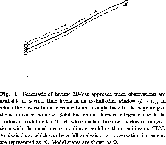
If there are data at different time levels we can choose to bring the data increments to the same initial time level (as shown schematically in Fig. 1) so that the increments corresponding to the different data can be averaged, with weights that may depend on the time level or the type of data. For applications in which ``knowing the future'' is allowed, such as reanalysis, the observational increments could be brought to the center of an interval, and used for the final analysis. In section 4 we show that, in a simple nonlinear model with complete data, when increments are brought to the same initial time, we solve a separate minimization for each time level, but that in fact (at least for this model) the I3D-Var minimizes the same multiple-level cost function as the simplified 4D-Var problem.

3. Burgers' equation example

a. Simple TLM, adjoint and inverse model formulation

Consider the simplest example of a model with advection of a passive scalar and diffusion, based on Burgers' equation

$$\left. \begin{array} {c} \frac{{\partial}{\overline{u}}}{{\... ...ial^{2}}{\overline{q}}}{{\partial}{x^{2}}} \end{array} \right.$$ (16)

where

$${\overline{u}} = u + {{\delta}u}, ~~~~~~~ {\overline{q}} = q + {{\delta}q},$$

${\nu}_{1}$ and ${\nu}_{2}$ are diffusion coefficients, and we assume that the basic flow u(x) and q(x) are slowly varying functions of x, and neglect their time changes.

The linear perturbation model is then

$$\left. \begin{array} {c} \frac{{\partial}{{\delta}u}}{{\par... ...rtial^{2}}{{\delta}q}}{{\partial}{x^{2}}}. \end{array} \right.$$ (17)

Assume

$${{\delta}u} = A(t)e^{ik(x-ut)}.$$

Then

$$\frac{dA}{dt} - ikuA = -ikuA - A{\frac{du}{dx}} - {\nu}_{1}{k^{2}}A$$

or

$$A(t) = A_{0}e^{-({\frac{du}{dx}}+{\nu}_{1}{k^{2}})t}.$$ (18)

We can interpret the first term in the exponent as an instability associated with the large scale flow (perturbations grow where there is convergence, ${\frac{du}{dx}}<0$), whereas the second term represents small scale dissipative processes. The imaginary exponent represents the effects of large scale advection.

Assume

$${{\delta}q} = B(t)e^{ik(x-ut)}.$$

Then, replacing, we find a diagnostic relationship between ${{\delta}q}$ and ${{\delta}u}$:

$$B(t) = \frac{{\frac{dq}{dx}}}{{\frac{du}{dx}}+({\nu}_{1}+{\nu}_{2}){k^{2}}}A(t).$$ (19)

So the solution is

$${{\delta}u}(t) = e^{-ikut}e^{-{\frac{du}{dx}}t}e^{-{\nu}_{1}{k^{2}}t}{{\delta}u}(0)$$ (20)

which can be interpreted as

final perturbation = (large scale advection)(large scale instability)(diffusion)initial perturbation.

The equation for ${{\delta}q}(t)$ is the same as ${{\delta}u}(t)$, except that ${{\delta}q}$ is also related to ${{\delta}u}$ by the diagnostic relationship given in (19).

The Tangent Linear Model (TLM) or propagator between time=0 and time=t, is then

$$L = e^{-({\frac{du}{dx}}+{\nu}_{1}{k^{2}})t-ikut}.$$ (21)

The adjoint model is obtained by taking the complex conjugate of the transpose:

$$L^{*}~=~e^{-({\frac{du}{dx}}+{\nu}_{1}{k^{2}})t+ikut}.$$ (22)

The exact inverse linear tangent model is obtained by integrating backwards in time (changing the sign of time):

$$L^{-1}~=~e^{({\frac{du}{dx}}+{\nu}_{1}{k^{2}})t+ikut}$$ (23)

and the approximate inverse (quasi-inverse) QTLM (Pu et al. MWR 1997) is obtained by integrating backwards in time except for changing the sign of the diffusion terms:

$$L^{\prime}~=~e^{({\frac{du}{dx}}-{\nu}_{1}{k^{2}})t+ikut}.$$ (24)

If we integrate forward with the linear model followed by a backward integration with the exact inverse we get the exact initial conditions:

L^-1L = I.

If we integrate forward with the linear model followed by a backward integration with the adjoint, the unstable modes grow both during the forward and the backward integration, and damping also occurs twice:

$$L^{*}L~=~e^{-2({\frac{du}{dx}}+{\nu}_{1}{k^{2}})t},$$ (26)

whereas if we follow the forward integration with a backward integration with the quasi-inverse QTLM, we get:

$$L^{\prime}L~e^{-2{\nu}_{1}{k^{2}}t},$$ (27)

i.e., we get the exact initial condition except smoothed twice by the diffusive terms.

b. Application of 4D-Var and Inverse 3D-Var to Burgers'’ equation

Let us assume that $\mathsf{H}=I$ (observations are made in the model variable space), and neglect for the moment diffusion terms. Then

$${{\delta}q}(t)~=~{\frac{dq}{du}}{{\delta}u}(t),$$

and it seems natural to assume

$$B~=~\frac{1}{\alpha} \left[ \begin{array} {cc} 1 & 0 \\ ... ...cc} 1 & 0 \\ 0 & \frac{Q^{2}}{U^{2}} \end{array} \right],$$ (28)

where $\alpha$, $\beta$ are appropriate scaling factors, and U², Q²are observational error variances, and (dq/du)² represents the ratio of the variance of q and u in the mean flow.

Then, from (10), the Inverse 3D-Var analysis is given by

$$L \left( \begin{array} {c} {{\delta}u} \\ {{\delta}q} \en... ...)^{2} \frac{Q^2}{U^2}+1}{{\delta}q}^{obs} \end{array} \right),$$ (29)

where $\gamma$ = $\alpha$/$\beta \gg$ 1 corresponds to small background errors (good forecast) and $\gamma \ll$ 1 to a poor forecast. Therefore the Inverse 3D-Var solution is

$$\left( \begin{array} {c} {{\delta}u} \\ {{\delta}q} \end{... ...)^{2} \frac{Q^2}{U^2}+1}{{\delta}q}^{obs} \end{array} \right).$$ (30)

The observational increments are appropriately weighted and moved back in time (advected and decreased where the flow is unstable). Note that in areas of large-scale decay (${\frac{du}{dx}}\gt$) the initial increments will be larger than at the final time and vice versa. This is not of concern, because when integrated forward, they will decay to their proper observed values.

The first iteration of the regular 4D-Var, on the other hand, is:

$$\left( \begin{array} {c} {{\delta}u} \\ {{\delta}q} \end{... ... {{\delta}u}^{obs} \\ {{\delta}q}^{obs} \end{array} \right)$$ (31)

where a is an appropriately chosen amplitude. Like the forecast sensitivity problem, it moves the observational increment backward in time, but enhancing the growing modes during the adjoint integration. It should be noted that when the 4D-Var is iterated, eventually it should converge to the same solution (30).

4. Numerical experiments

We have performed preliminary experiments with the NCEP global model (Pu et al. 1997a), and with two simple models, the Lorenz (1963) model and Burgers' equation with passive transport.

a. The NCEP global model

The application to the global NCEP model was a forecast sensitivity approach. The 24 hour forecast error was estimated from the 24-hour analysis, and the difference between the analysis and the forecast was integrated backwards, using the TLM of the NCEP global model, with the sign of surface friction and horizontal diffusion changed. The results were very encouraging, indicating that the correction of the forecast was considerably better than using the adjoint sensitivity approach, even when the latter was iterated 5 times (Pu et al. 1997a). Several important points should be noted:

a)

Ideally, the TLM integrated backwards should have a reversible formulation of the Hamiltonian (energy conserving) dynamics. In practice, the NCEP model has only approximately reversible dynamics (e.g., the Robert time filter is slightly diffusive). This will introduce additional diffusion during the backward integration; this subject is further discussed in the next sub-section.

b)

A known nonlinear solution was integrated backward and again forward over 24 hours. The error in reproducing the full nonlinear perturbation with the TLM and the quasi-inverse TLM was about 10 % in both total and kinetic energy throughout the model atmosphere, except near the surface, where the effect of changing the sign of friction is most important and where the error reached about 25 %.

c)

The amplitude of the quasi-inverse sensitivity was much larger than the adjoint sensitivity. This is because the adjoint sensitivity focuses only on the fastest growing modes (cf. Eq. 26), whereas the quasi-inverse sensitivity includes both growing and decaying modes (and the latter grow during the backward integration). This may result in unwanted noise growth, and needs to be handled carefully.

b. Burgers' equation with advection of a passive scalar

We performed some numerical tests with Burgers' equation including advection of a passive scalar (16). It should be noted that the model had been originally programmed using the Lax scheme (e.g., Anderson et al. 1984), which is highly diffusive and far from reversible (S. K. Park, personal communication, 1998). Such a scheme would not be appropriate for a method that requires approximating the inverse of the model by running it backwards. This was easily solved by rewriting the model with a leapfrog scheme for advection (with a forward first time step) and DuFort-Frankel for diffusion (e.g., Anderson et al. 1984). Therefore the numerical scheme was fully reversible except for the first forward time step. This allowed us to compare the effects of using the exact inverse linear model (IL) and the quasi-inverse linear model (QIL) as long as the Reynolds number was large enough (i.e., low dissipation) for the exact inverse to remain computationally stable.

The results were excellent. Fig. 2a shows the cost function for a case in which the first guess included errors of 50 %, and the observations were exact. As in Wang et al. (1997), the observation field at the end of the assimilation interval was complete, and the cost function did not include a background term. Unless noted otherwise, the results described below are computed with the QIL. The 4D-Var minimization was performed using the LBFGS algorithm (Liu and Nocedal 1989), based on a limited-memory quasi-Newton method. It should be noted that the parameter for checking directional derivative condition (GTOL) in the LBFGS algorithm has to be chosen appropriately for each problem; after some experimentation, we chose it to be GTOL=0.1, which we found to be optimal for the 4D-Var in our case.

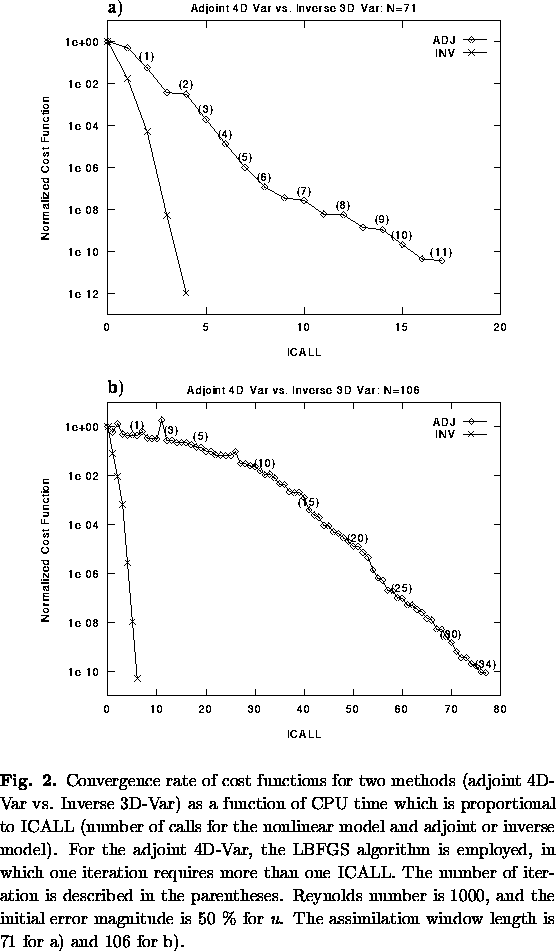
For an assimilation window of 71 time steps, the Inverse 3D-Var converged to less than 10^-12 of its initial value in 4 iterations, whereas the adjoint algorithm required 11 iterations (and 17 computations of the gradient, each one involving a forward and backward integration) in order to converge to 10^-10. For longer assimilation windows, the advantages of Inverse 3D-Var became more apparent. For example, when the assimilation window was extended to 106 time steps (Fig. 2b), Inverse 3D-Var converged to 10^-10 in only 5 iterations. The 4D-Var, on the other hand, converged to the same value in 34 iterations, and almost 80 computations of the gradient (each one involving a forward and backward integration of the model or its adjoint). Choices of smaller GTOL resulted in a lack of convergence.

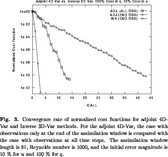
In Fig. 3 we have included passive transport of a scalar, with 10 % errors in the initial velocities u, and 100 % errors in q. For an assimilation window of 81 time steps, the Inverse 3D-Var converges to 10^-13 of its original value after 3 iterations, but 4D-Var with data at the end of the interval requires 44 equivalent model integrations to converge to 10^-10. If we provide 4D-Var with observations for every time step, it converges to 10^-10 of the original cost function in 12 time integrations.

Many other experiments including observational and background errors were performed with uniformly good results. Some of the conclusions from these experiments (S. K. Park, personal communication, 1998) are:

a)

Results from Inverse 3D-Var are very good in essentially every case. In general, for large Reynolds number (low dissipation), the QIL converges slightly faster than the exact IL. For small Reynolds number, the IL becomes unstable, but the QIL still converges fast.

b)

We also tested the results of having multiple time levels in the observations. We included random errors in the observations with maximum amplitude of 10% of the total range. We followed the approach of Fig. 1, i.e., we brought the observational increments (innovations) from different observational times backwards to the same initial time level. Performing an average of the simultaneous increments gives very good results, and improves forecasts beyond the assimilation window roughly like 1/$\sqrt{n}$, where n is the number of time levels in the observations. Additional iterations are performed integrating the nonlinear model from the updated initial conditions, and integrating backwards the observational increments. The results of the forecasts with one iteration of Inverse 3D-Var were comparable to those of 20 iterations of 4D-Var, whereas 3 iterations of Inverse 3D-Var resulted in much better forecasts (Fig. 4).

c)

It is important to note that in this experiment, the Inverse 3D-Var approach in practice minimizes the same total cost function as the variational approach, even though it is only guaranteed to minimize one observation level at a time (Table 1). The variational approach gives a slightly better minimization after 4 iterations, but this does not translate into a more accurate forecast (Fig. 4, verified against truth), since there is slight overfitting of noisy observations.

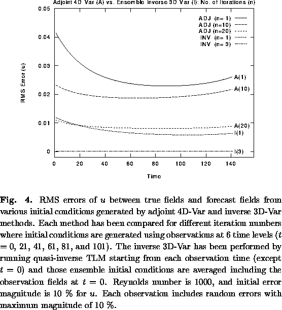
Table 1. Variations in the cost function computed from different initial conditions generated by the same procedure as in Fig. 4 except that each 4D-Var (adjoint and ensemble inverse) has stopped at iteration numbers of 1 to 5.

Iteration Adjoint Ensemble Inverse

0 41.8588 41.8588

1 22.5407 1.7420

2 2.1480 0.9197

3 2.0967 0.8881

4 0.8558 0.8787

5 0.8666 0.8746

c. Experiments with Lorenz 3 variable model

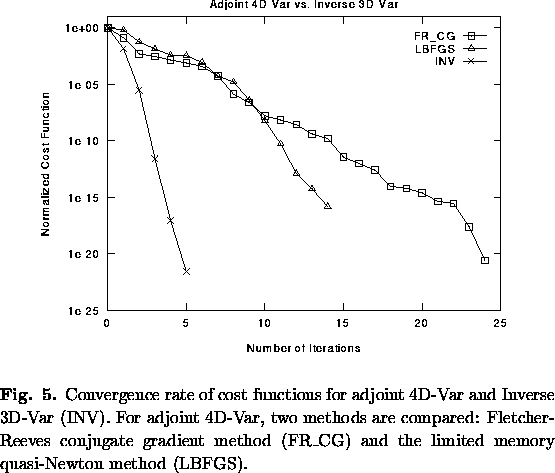
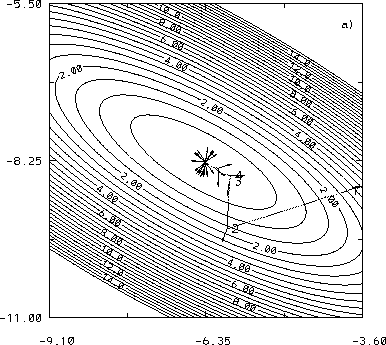
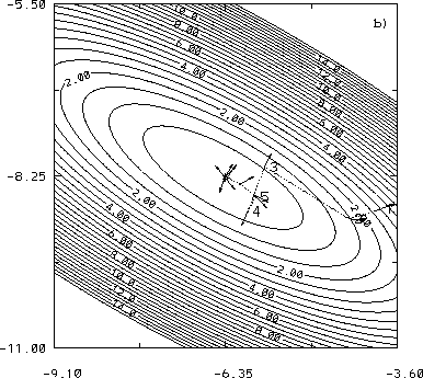
Inverse 3D-Var was also tested and compared with regular (adjoint) 4D-Var using Lorenz (1963) 3-variable model. Fig. 5 shows the evolution of the cost function using two different library minimization algorithms for the 4D-Var approach (limited-memory quasi-Newton or LBFGS, and Fletcher-Reeves conjugate gradient or FR_CG - see Navon and Legler (1987) for details) and the Inverse 3D-Var. The results are similar to those obtained with Burgers' equation: Inverse 3D-Var reduces the cost function to 10^-10 in 3 iterations and to 10^-22 in 6 iterations. The conjugate gradient and quasi-Newton methods converge to 10^-14 in about 20 and 14 iterations respectively (where each iteration includes several forward nonlinear and backward adjoint integrations). Fig. 6 shows the cost function in the (X₀,Y₀) space and the descent approach of the 3 algorithms. The fact that Inverse 3D-Var is equivalent to a Newton algorithm is apparent by the directness of its convergence: both the descent direction and the amplitude of the step are optimal.

Several additional experiments with random errors in the initial conditions, multiple levels of observations, and observations of subset of variables and their combinations have also given uniformly excellent results (J. Gao, personal communication, 1998).

5. Discussion

In the following discussion we first consider the relationship between the traditional 6-hour cycle for 3D-Var, 4D-Var, and Inverse 3D-Var (Cohn 1997; Courtier 1997). In 3D-Var (or previously in Optimal Interpolation) the observations were lumped together within a $\pm$3-hour window, and were assumed to have been taken at the center of the interval. For example, an analysis at 12Z included observations taken between 9Z and 15Z, but assumed to be observed at 12Z. For observations made, for example, at 10Z, this introduces two (relatively small) errors: the innovations (observations minus background) are computed with respect to a forecast at the wrong time, and the innovations are applied at the wrong time (12Z instead of 10Z). The first error can be easily corrected within 3D-Var: the background can be computed at the time of the observation, rather than at the center of the window. This correction is currently done at NCEP. However, only 4D-Var corrects the second error. 4D-Var (as implemented at ECMWF) computes the initial conditions valid at 9Z that best fit the data at their correct times throughout the 9Z-15Z interval. It minimizes a cost function that includes distance to the background at 9Z, plus the distance to the observations at their correct time (binned into one hour intervals). The 4D-Var ``analysis'' at 12Z is defined as the 3-hour forecast from the optimal initial conditions at 9Z. Because the minimization required about 80 iterations before reaching a satisfactory level, ECMWF has used a T63 model for the minimization, whereas the forecast model has T213 resolution.

Inverse 3D-Var offers some additional flexibility: If observations are complete, it allows transporting all the innovations from 9Z to 15Z to the desired time (12Z) essentially exactly (Fig. 1). The innovations at 12Z can then be analyzed into a 3D-Var that includes different background weights depending on the length of the forecast. In general, however, the observations are not complete, and a background error covariance needs to be introduced into the cost function. In that case, the Inverse 3D-Var analysis at the end of the assimilation interval is equivalent to 3D-Var, but the analysis is reached through a model integration, which can be advantageous in reducing problems of spin up. When knowledge of ``future'' observations is available (as in reanalysis), and the goal is to optimize the analysis (rather than to improve the forecast), the Inverse 3D-Var can also be used, as suggested by the forecast sensitivity applications.

We have seen that Inverse 3D-Var has several potential advantages, including accuracy, efficiency and flexibility, and these have been apparent in the simple model experiments. It also has some potentially serious disadvantages, but we believe they can be overcome with further development and experimentation:

a)

Growth of noise that projects on decaying modes during the backward integration. This is a very serious problem, but it need not be a ``show-stopper'' since those errors will decay again during the next forward integration. The results of Pu et al. (1997a) for integrations 24 hour and longer, and those obtained here with the Burgers' equation and observational noise are quite encouraging in this respect. It should be noted that the results obtained by Reynolds and Palmer (1998) when studying this problem are in full agreement with those of Pu et al. (1998) and of the present paper. They found that analysis uncertainties grew during the backward integration, but that during the forward integration they decayed again. As a result the forecast error reduction achieved at the end of the interval using the Quasi-Inverse was equivalent to that derived using the Pseudo-Inverse method with 60 to 90 Singular Vectors, but it was obtained at a computational cost several orders of magnitude smaller.

b)

Physical processes are generally not parameterized in a reversible form in atmospheric models. This is also serious, but to some extent it can be overcome. For example, moist convective processes can be simplified and parameterized in a reversible manner through the first hour of model integration (Jerry Straka, pers. comm., 1998). We are testing this idea with the ARPS model, where we plan to use a reversible parameterization of convection to ``phase correct'' the background field when, for example, the model predicts a squall line shifted in space and time from the observations.

c)

The basic hydrodynamics of a model may not be written in a reversible fashion. If the numerical discretization of the hydrodynamics is excessively dissipative, this may require some rewriting, as discussed in section 4. Slightly dissipative schemes, when integrated backwards will also fall within the ``QIL'' approach: they will dissipate both forward and backwards.

d)

The truly dissipative processes in the atmospheric model are not reversible, or may be reversible only for short intervals. If dissipation is a major factor during an assimilation window, it will not be well represented by Inverse 3D-Var. On the other hand, both our results and those of Reynolds and Palmer (1998), suggest that in most cases, the quasi-inverse approximation slightly improves the results.

e)

Finally, it has to be demonstrated with more complex systems that in nonlinear integrations this method will provide an improvement upon what can be attained with 3D-Var alone.

We are currently planning to test the Inverse 3D-Var approach on the ARPS model, by combining it with a 3D-Var analysis including Doppler radar observations of radial velocities and reflectivities, using a linear tangent model with simplified reversible physics. If successful, we will also attempt to apply this method to the NCEP global model, where it could be applied, for example, in the second phase of the global Reanalysis project (Kalnay et al. 1996), where ``future'' data is available during the assimilation.

Acknowledgments. This work was started at NCEP's Environmental Modeling Center. We would like to express our special gratitude to David Zhi Wang and his co-authors, for introducing similar ideas on the acceleration of 4D-Var, and Jerry Straka for developing a reversible parameterization of convection. Discussions with Kelvin Droegemeier, Keith Brewster, Alan Shapiro and Brian Fiedler at the University of Oklahoma, Mark Iredell, Wan-Shu Wu, Zoltan Toth, M. Zupanski, D. Zupanski at NCEP, R. Menard and S. Cohn at NASA/DAO, Carolyn Reynolds, Tim Palmer, and Michael Navon were also helpful. We are especially grateful to Olivier Talagrand, Andrew Lorenc, Francois Bouttier, Istvan Szunyogh, Jim Purser, John Derber and David Parrish for their insightful comments on an early version of the paper.

The support and encouragement of Peter Lamb (CIMMS), Kelvin Droegemeier (CAPS), and Fred Carr (School of Meteorology), and Ron McPherson and Stephen Lord (NCEP) are gratefully acknowledged. This research was supported by DOC/NOAA under Grant NA67J0160 through CIMMS and NSF under Grant ATM91-20009 through CAPS.

7. References

Anderson, D. A., J. C. Tannehill, and R. H. Pletcher, 1984: Computational Fluid Mechanics and Heat Transfer. Hemisphere Publishing Corp., 599 pp.

Bouttier, F., and F. Rabier, 1997: The operational implementation of 4D-Var. ECMWF Newsletter, No. 78, 2-5.

Cohn, S. E., 1997: An introduction to estimation theory. J. Meteor. Soc. Japan, 75 (1B), 257-288.

Courtier, P., 1997: Variational methods. J. of Meteor. Soc. of Japan, 75 (1B), pp 211-218.

     , J.-N. Thepaut, and A. Hollingsworth, 1994: A strategy for operational implementation of 4D-Var using an incremental approach. Quart. J. Roy. Met. Soc., 120, 1367-1388.

Daley, R., 1991: Atmospheric Data Analysis. Cambridge University Press, 457 pp.

Derber, J. C., 1989: A variational continuous assimilation technique. Mon. Wea. Rev., 117, 2437-2446.

Gill, P. E., W. Murray and M. H. Wright, 1981: Practical Optimization. Academic Press, pp 401.

Ide, K., P. Courtier, M. Ghil and A. Lorenc, 1997: Unified notation for data assimilation: operational, sequential and variational. J. of Meteor. Soc. Japan, 75 (1B), pp 181-197.

Kalnay, E., and Z.-X. Pu, 1998: Application of the quasi-inverse method to accelerate 4D-Var. Preprints, 12th Conf. on Numerical Weather Prediction, Phoenix, AZ, Amer. Meteor. Soc., 41-42.

     , M. Kanamitsu, R. Kistler, W. Collins, D. Deaven, L. Gandin, M. Iredell, S. Saha, G. White, J. Woollen, Y. Zhu, M. Chelliah, W. Ebisuzaki, W. Higgins, J. Janowiak, K. C. Mo, C. Ropelewski, J. Wang, Leetmaa, R. Reynolds, Roy Jenne, and Dennis Joseph, 1996: The NCEP/NCAR 40-year Reanalysis Project. Bull. Amer. Meteor. Soc., 77, 437-471.

Le Dimet, F.-X., and O. Talagrand, 1986: Variational algorithms for analysis and assimilation of meteorological observations: Theoretical aspects. Tellus, 38A, 97-110.

Lewis, J. M., and J. C. Derber, 1985: The use of adjoint equations to solve a variational adjustment problem with advective constraints. Tellus, 37A, 309-322.

Lorenc, A. C., 1988: A practical approximation to optimal four-dimensional objective analysis. Mon. Wea. Rev., 116, 730-745.

Lorenz, E. N., 1963: Deterministic nonperiodic flow. J. Atmos. Sci., 20, 130-141.

Menard, R., and R. Daley, 1996: The application of Kalman smoother theory to the estimation of 4DVAR error statistics. Tellus, 48A, 221-237.

Molteni, F., R. Buizza, T. N. Palmer, and T. Petroliagis, 1996: The ECMWF Ensemble Prediction System: Methodology and validation. Quart. J. Roy. Meteor. Soc., 122, 73-119.

Navon, I. M., and D. M. Legler, 1987: Conjugate-gradient methods for large-scale minimization in meteorology. Mon. Wea. Rev., 115, 1479-1502.

Pires, C., R. Vautard, and O. Talagrand, 1996: On extending the limits of variational assimilation in monlinear chaotic systems. Tellus, 48A, 96-121.

Pu, Z.-X., E. Kalnay, J. Sela, and I. Szunyogh, 1997a: Sensitivity of forecast errors to initial conditions with a quasi-inverse linear model. Mon. Wea. Rev., 125, 2479-2503.

     ,      , J. Derber and J. Sela, 1997b: An inexpensive technique for using past forecast errors to improve future forecast skill. Quart. J. Roy. Met. Soc., 123, 1035-1054.

     , S.J. Lord and E. Kalnay, 1998: Forecast Sensitivity with dropwindsonde data and targeted observations. Tellus, 50A, 391-410.

Rabier, F., E. Klinker, P. Courtier and A. Hollingsworth, 1996: Sensitivity of forecast errors to initial conditions. Quart. J. Roy. Meteor. Soc., 122, 121-150.

     , J.-F. Mahfouf, M. Fisher, H. Järvinen, A. Simmons, E. Andersson, F. Bouttier, P. Courtier, M. Hamrud, H. Haseler, A. Hollingsworth, L. Isaksen, E. Klinker, S. Saarinen, C. Temperton, J.-N. Thepaut, P. Undén and D. Vasiljevic, 1997: The ECMWF operational implementation of four-dimensional variational assimilation. ECMWF Research Department Tech. Memo., No. 240.

Reynolds, C. and T. N. Palmer, 1998: Decaying singular vectors and their impact on analysis and forecast corrections. J. Atmos. Sci., 55, 3005-3023.

Rohaly, G. D., R. H. Langland, and R. Gelaro, 1998: Identifying regions where the forecast of tropical cyclone tracks is most sensitive to initial condition uncertainty using adjoint methods. Preprints, 12th Conf. on Numerical Weather Prediction, Phoenix, AZ, Amer. Meteor. Soc., 337-340.

Thepaut, J.-N., R. N. Hoffman and P. Courtier, 1993: Interactions of dynamics and observations in a 4-dimensional variational assimilation. Mon. Wea. Rev., 121, 3393-3414.

Wang, Z., K. K. Droegemeier, L. White and I. M. Navon, 1997: Application of a New Adjoint Newton Algorithm to the 3D ARPS Storm-Scale Model Using Simulated Data. Mon. Wea. Rev., 125, 2460-2478.

     , I. M. Navon, X. Zou, and F. X. Le Dimet, 1995: A truncated Newton optimization algorithm in meteorology applications with analytic Hessian/vector products. Computational Optimization and Applications, 4, 241-262.

Xue, M., K. K. Droegemeier, V. Wong, A. Shapiro, and K. Brewster, 1995: ARPS Version 4.0 Users' Guide. Center for Analysis and Prediction of Storms, University of Oklahoma, 380 pp. [Available from Center for Analysis and Prediction of Storms, University of Oklahoma, Norman, OK, 73019.]

Zupanski, D., 1997: A general weak constraint applicable to operational 4DVAR data assimilation systems. Mon. Wea. Rev., 125, 2274-2292.

Zupanski, M., 1993: Regional 4-dimensional variational data assimilation in a quasi-opera- tional forecasting environment. Mon. Wea. Rev., 121, 2396-2408.